Simulating Performance

Navigation: Analysing with algorithms > Simulators >

Background

The architectural evaluator for performance is a discrete event simulator that works by simulating the flow of messages (or tokens) throughout an architecture. The theory behind this is derived from research done by the University of Technology, Sydney, and is based on Layered Queuing Network Models (LQNM), Timed and Coloured Petri-Nets (TCPN) and Activity Cycle Diagrams (ACD).

In the ABACUS performance simulation, processing on one component is driven largely by messages passed to it from another component. The principles behind this technique can be understood in four main parts:

1.The message-centric communication is modelled in ABACUS using logical (or indirect) connections. Logical connections define the performance (frequency and data) of the messages passed between the components. A good example of logical connections would be the sequence flows between two (2) business processes or the logical interfaces between two (2) applications.

2.Logical messages are transported to their destination via hierarchy (such as resource swimlanes) or direct connections (such as physical wires). To do this they can be routed up, across and back down the hierarchy (a layered approach) to follow the direct path.

3.The fidelity of the model can be adjusted to suit. For example, a process can be divided down so far such that each elementary process and function has a separate processing footprint. Alternatively, it may be enough to have just one value for the entire process, reflecting the average processing response to a message.

4.The actual processing is performed only by components that have (or are) a processor. A processor is a generic thing, and could be a CPU, a person, an organisational unit or anything else that is capable of carrying out work. For example, a business process does not do any actual processing; this is done by the first ‘processor’ it locates in either its parent hierarchy (if a swimlane notation is used) or its processing network (if a distributed processing notation is used).

The evaluation is performed by simulating the (specified) traffic in the system, such that every connection is simulated at least once. Arrival times of messages are randomly generated with regard to their specified frequency. The model simulates resource processing and contention and the queuing of messages, gathering statistics along the way as various output properties.

Key Performance Input Factors

1.Frequency – The frequency at which the connection occurs.

2.Processing – The amount of execution time to complete one process. This may be in hours, minutes, days, operations etc.

3.Speed – The speed of the processor resource. That is, how many cycles / instructions / actions it can perform in one unit of time. It is important to be consistent with the units used for Processing.

4.Processors – The number of processor resources. Processors could be people, CPU’s, external organisations etc.

Key Performance Output Factors

1.Throughput – The number of messages per time unit through the connection. This actual value may be compared with the expected/theoretical values (i.e. Frequency) to deduce saturation of the system.

2.Message Rate – The number of messages per time unit through the component. This is the sum of all the components' incoming and outgoing messages.

3.Response – The minimum / average / maximum latency for this connection. This is the sum of all the observed latencies for the connection from the source to the sink and any queuing and processing (and latency back to the source if bidirectional).

4.Utilisation – The utilisation of the component. This will be 0% if the component is not a device/processor (i.e. it does not have the Processors and Speed properties defined above).

While a discrete event simulation is performed to calculate the various output properties, as described above, the following formula may be used as a rough verification of the results (where the system is not saturated):

Utilisation = Sum of Frequency for all incoming connections * Processing / (Speed * Processors)

The overall concept is perhaps best demonstrated by considering the following diagram, which shows two different performance metamodels. The left hand style is the classic ‘swimlane’ notation with processing tasks based hierarchically within their processor resources. The right hand style is a ‘distributed’ notation with the processing tasks connected via a processes connection to their processor resource. This latter notation allows multiple processor resources for a given processing task, unlike the limited swimlane notation.

Note

Shown on each metamodel are the input properties (in red) and output properties (in blue):

Performance metamodels: Swimlane versus Distributed notation

Running the Performance simulator

To simulate your architecture in terms of performance

1.Ensure you have the ABACUS file, containing your populated architecture, open.

2.Select Analysis | Performance or click the toolbar button.

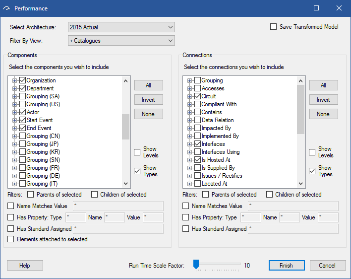
3.Select the Architecture you wish to evaluate from the pull-down menu.

Note

By default, ABACUS will automatically select the first architecture for which a re-simulation is required due to any underlying property or structural changes. This highlighting is shown in Red on the Simulation toolbar.

4.Select the Components and Connections you wish to evaluate, from the standard element selection window.

5.Set the Run Time Scale Factor slider.

Note

Higher values will yield more statistically consistent results but take longer time to calculate.

Additional Checkbox to the standard element selection window

•Save Transformed Model will save a copy of the RBD transformed version of the project in the same folder as the current project and append "_transformed" to the project name. This transformed project can be used to diagnose in detail the reliability simulation undertaken by ABACUS.

Other options to the standard element selection window

•Run Time Scale Factor controls the simulation time and accuracy with higher values yielding more statistically consistent results but taking longer time to run.

Note

When ABACUS calculates the simulation time it will determine the slowest indirect connection Frequency that was selected to be simulated and then 'warm-up' for the Period (i.e. 1 over the Frequency) of this connection (initiating periodic message generators for all the connections randomly during this warm-up time, giving them all a chance to initiate) and then simulate for Run Time Scale Factor times the Period of that connection. Or (1 / Frequency) warm-up time + (1 / Frequency) * Run Time Scale Factor simulation time. This is to make sure that that all the connections are initiated before statistics are collected and then the slowest connection is still simulated at least once in the simulation. E.g. If the slowest indirect connection has a Frequency of 0.033 time-units (or circa once a month if the time-units are days) then the warm-up time will be 30.3 time-units and the simulation time will be 30.3 time-units times the Run time Scale Factor.

6.Click Finish and you will get a Warning dialog.

7.Optionally explore the warnings by clicking Details >>.

8.Click Continue.

Note

At this point, ABACUS will perform a discrete-event simulation of the architecture and after a short time (with progress bars for feedback) a calculation complete dialog will appear.

9.Click OK to acknowledge the simulation.

Tip

For training courses and further help on Performance Simulation please refer to the Avolution Community.

Component Properties

The following table lists the properties required to evaluate performance. Properties are searched for first in the Component instances, then the Component Standards and if not found, the default is used. These properties will be shown in the Properties window with a property input row selector icon () with the tooltip 'Performance Input'. A change to any of these 'input' properties and various structural changes to the repository will result in the Performance simulator requiring a re-simulation as indicated in Red on the Simulation toolbar.

Type	Name	Default Value	Unit	Data Type	Required	Description
Performance	b_pack	0.0		Decimal	False	The fixed service time to pack in seconds. This property is typically specified as an standard type and then used for multiple component instances. For example, CORBA has b_pack = 0.23 ms.
Performance	m_pack	0.0		Decimal	False	The variable service time to pack in seconds / byte. This property is typically specified as an standard type and then used for multiple component instances.
Performance	b_unpack	0.0		Decimal	False	The fixed service time to unpack in seconds. This property is typically specified as an standard type and then used for multiple component instances.
Performance	m_unpack	0.0		Decimal	False	The variable service time to unpack in seconds / byte. This property is typically specified as an standard type and then used for multiple component instances.
Performance	Processing	0.0		Decimal	True	The amount of execution time to complete one process. This may be in hours, minutes, days, operations etc.
Performance	Processors	1		Integer	True	The number of Processor resources. Processors could be people, CPU’s, external organisations etc.
Performance	Speed	100		Integer	True	The speed of the processor resource. That is, how many cycles / instructions / actions it can perform in one unit of time. It is important to be consistent with the units used for Processing.
Performance	k_bkgd	0.0		Decimal	False	Background processing on the component. This is used to adjust the results to match any fixed offsets for %. This can probably be ignored.

The following table lists the component properties output by the performance evaluator. A set of these component properties are generated for each component on each performance run. These properties will be shown in the Properties window with a property output row selector icon () with the tooltip 'Performance Output'. The arrow on the icon will highlight Red () when these properties are out of date due to an underlying property or structural change to the repository and the Performance simulator requires re-simulation according to the Red highlighting on the Simulation toolbar.

Type	Name	Unit	Data Type	Required	Description
Performance	Message Rate		Decimal	False	The number of messages per time unit through the component. This is the sum of all the components' incoming and outgoing messages.
Performance	Bandwidth		Decimal	False	Overall bandwidth through the component. The sum due to both incoming and outgoing messages.
Performance	Utilisation	%	Decimal	False	The utilisation of the component. This will be 0% if the component is not a device/processor (i.e. It does not have Processors and Speed properties defined above)

Connection Properties

The following table lists the properties required to evaluate performance. Properties are searched for first in the Connection instances, then the Connection Standards and if not found, the default is used. These properties will be shown in the Properties window with a property input row selector icon () with the tooltip 'Performance Input' or 'Financial/Performance Input'. A change to any of these 'input' properties and various structural changes to the repository will result in the Performance simulator and/or Financial simulator requiring a re-simulation as indicated in Red on the Simulation toolbar.

Type	Name	Default Value	Unit	Data Type	Required	Description
Performance	Kind	bidirectional	[bidirectional \| unidirectional]	Lookup / List	True	Whether the connection is two-way (bidirectional) or one-way (unidirectional). The allowed values for this property are "bidirectional" or "unidirectional". Bidirectional means synchronous request / response messages whereas unidirectional means a single asynchronous "event".
Performance	Abstraction	indirect	[indirect \| direct]	Lookup / List	True	Whether the connection is physical or logical. Direct connections are physical "pipes" between two components that logical connections flow along. The allowed values for this property are "direct" or "indirect". If the value is "direct" then the connection does not need any other properties (except for the properties Kind and Abstraction).
Performance	L_app1	0		Integer	False	Request / event size in bytes. Every connection will typically have a specific value for this. In CORBA, events are actually bidirectional and always have a 12 byte acknowledge (L_app2). If it is a true unidirectional connection then leave out the property L_app2.
Performance	L_app2	0		Integer	False	Response / acknowledge size in bytes. Every connection will typically have a specific value for this. A unidirectional connection will not have L_app2.
Performance	Frequency	1		Decimal	True	The frequency at which the connection occurs. Every connection will typically have a specific value for this. If the property Frequency is left out then the default is used.
Performance	Relationship	processes	[processes \| supports]	Lookup / List	False	Connections that have the "processes" property indicate that the component at the start of the connection will be transformed to be processed at the component at the end of the connection. In effect the "source" component is moved to become a child of the "sink" component (the attached connections are also "dragged" with this move). If a "processes" property exists then all the other connection properties will be ignored, except the optional "%" property described below.
Performance	%	100.0		Decimal	False	Connections that have the "processes" property (described above) can optionally have a "%" property to indicate the proportion of the processing that will be attributed to the destination component. In this way a single source component can be processed by multiple destination components at various %'s. The % values do not need to add up to 100% and it is simply used to scale the "processing" property (see above) for the source component as it is transformed to become a child of the destination component.

The following table lists the properties generated by the performance evaluator. A set of these connection properties are generated for each connection on each performance run. These properties will be shown in the Properties window with a property output row selector icon () with the tooltip 'Performance Output'. The arrow on the icon will highlight Red () when these properties are out of date due to an underlying property or structural change to the repository and the Performance simulator requires re-simulation according to the Red highlighting on the Simulation toolbar.

Type	Name	Unit	Data Type	Required	Description
Performance	Bandwidth		Decimal	False	The overall bandwidth for the connection. This is only calculated for indirect connections and is essentially (L_app1 + L_app2)*Throughput.
Performance	Bandwidth 1/2		Decimal	False	The bandwidth specifically for outgoing (1) and incoming (2) messages of the connection. This is only calculated for indirect connections and is essentially L_app1Throughput and L_app2Throughput.
Performance	Throughput		Decimal	False	The number of messages per time unit through the connection. This actual value may be compared with the expected/theoretical values (i.e. Frequency) to deduce saturation of the system.
Performance	Completed	%	Decimal	False	The percent of messages that successfully complete processing for the connection. This is only calculated for indirect connections and is the Throughput / Frequency. Occasionally the Completed value exceeds 100% because the randomness of message generation results in a slightly higher message generation frequency than specified.
Performance	Response (Min/Ave/Max)		Decimal	False	The minimum / average / maximum latency. This is only calculated for indirect connections and is the observed latency for the connection from source to sink and any queuing and processing (and latency back to the source if bidirectional).

Architecture Properties

The following table lists the system-wide architectural properties generated by the performance evaluator. A single set of properties for the architecture are "aggregated" for each performance run. These properties will be shown in the Properties window with a property output row selector icon () with the tooltip 'Performance Output'. The arrow on the icon will highlight Red () when these properties are out of date due to an underlying property or structural change to the repository and the Performance simulator requires re-simulation according to the Red highlighting on the Simulation toolbar.

Type	Name	Unit	Data Type	Required	Description
Performance	Message Rate		Decimal	False	The number of messages per time unit through the components in the architecture. This is the sum of all the components' incoming and outgoing messages.
Performance	Throughput		Decimal	False	The number of messages per time unit through the connections in the architecture. This is the sum of all the indirect connections' throughputs and this actual value may be compared with the expected/theoretical values (i.e. Frequency) to deduce saturation of the system.
Performance	Bandwidth		Decimal	False	The overall bandwidth. Sum of the architecture's connection bandwidths.
Performance	Utilisation	%	Decimal	False	The utilisation of all the components. Can be greater than 100% as it is just the sum of all the architecture's component utilisations.
Performance	Response (Min/Ave/Max)		Decimal	False	The minimum / average / maximum latency. Sum of all the observed latencies for the architecture's connections from source to sink (and back to source if bidirectional).